
The Blind Spot in Modern ML Monitoring
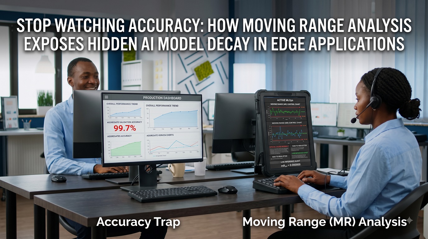
Your face verification model reports 96% accuracy. Users pass through your authentication flow smoothly. The system looks healthy.
Then an attacker runs a simple optimization attack against your live inference endpoint. Or an internal security patch introduces unexpected noise into the feature space. Or environmental drift—lighting changes, camera angles shifting subtly over time—begins to degrade predictions.
Your aggregate accuracy stays at 96%.
But something is wrong. The model’s confidence on individual predictions is bouncing erratically. One frame gives you 0.92 confidence, the next gives you 0.55, the next 0.94. The system is unstable—but you won’t know it by staring at your accuracy dashboard.
This is the fundamental problem with treating machine learning deployment like a static benchmark evaluation. You measure a single number—accuracy, F1 score, or precision—and assume that if it’s high, your system is safe. But production systems don’t live in static benchmarks. They live in time. They accumulate predictions. And over time, a model can develop serious pathologies while its average performance metric barely budges.
Why This Matters for Security and Reliability
Consider three concrete failure modes that plague production systems:
Model Decay from Adversarial Attack
An attacker runs targeted perturbations against your face authentication API. Each individual attack is subtle—confidence drops by a few percentage points on specific inputs. Aggregated across all predictions, the average barely moves. But for the handful of attackers trying to break in, the system is now predictably broken on certain inputs. Your 96% accuracy metric hides this targeted vulnerability.
Latent Feature Drift from Model Updates
You patch your model to fix a known vulnerability. The patch works—it blocks the specific attack. But it also changes the underlying feature representations in subtle ways. The model becomes noisier. Identical images produce slightly different predictions depending on initialization or hardware quirks. Over time, run-to-run variation increases even though aggregate accuracy stays stable.
Environmental Drift Without Clear Signals
Your deployment drifts into a regime where predictions are stable but less confident. Lighting changes, camera hardware upgrades, or seasonal environmental shifts cause the model to become more uncertain. The average accuracy doesn’t collapse—it’s still 94% or 93%—but the system has become fragile. One more environmental change, and it tips into failure.
Moving Beyond Static Metrics: Sequential Monitoring
The solution is not to add more metrics to your dashboard. It’s to stop treating inference as a collection of independent predictions and start treating it as a time series.
Industrial process control engineers solved this problem decades ago. In manufacturing, they don’t just measure whether your widget meets specification. They track how much each widget differs from the last one. When that “moving range” gets too large, it signals that something structural has shifted in the production process—even if the average product is still good.
We can apply the exact same logic to AI inference. Track the confidence score on each prediction. Look at how much it swings between consecutive predictions. If the swings get bigger than normal, something is wrong. This catches attacks, model updates, and environmental drift hours or days before aggregate metrics register the problem.
The DMAIC-GML Framework: Five Phases of Process Control
We apply Lean Six Sigma’s DMAIC methodology to deep learning inference, structured as five sequential phases:
Phase 1: Define — What Are We Measuring?
Instead of measuring aggregate accuracy, we measure the model’s confidence score on each inference. Call this X_t, the confidence at inference time t. More importantly, we measure the moving range—the absolute difference between consecutive predictions:
MRt = |Xt − Xt−1|
This single number tells you how stable the model is. High moving range means predictions are bouncing around unpredictably. Low moving range means the model is confident and consistent.
Phase 2: Measure — Establishing Normal Behavior
Run 30 inferences under clean, benign conditions. Calculate the average moving range (MR̄). Using standard statistical process control formulas, compute an upper control limit:
UCLMR = 3.267 × MR̄
Any moving range value above this limit is a red flag. It doesn’t necessarily mean an attack is happening. But it means something unusual is going on that deserves investigation.
Phase 3: Analyze — Understanding What Causes Variance
Run a controlled experiment varying three factors:
- Quantization (8-bit integers vs. 32-bit floating point)
- Architecture (fully connected classifier vs. global average pooling)
- Perturbation type (natural blur vs. adversarial gradient descent attack)
For each combination, measure the moving range. Use ANOVA to identify which architectural choices suppress noise. You’re essentially asking: which design decisions make the model more stable?
Phase 4: Improve — Hardening the Model
Based on the ANOVA results, lock in the architectural choices that minimize variance. For example, combining global average pooling with 8-bit quantization often reduces baseline noise significantly. Implement these changes. Your control limits (UCL_MR) shrink. The system becomes more sensitive to real anomalies because you’ve eliminated the background noise.
Phase 5: Control — Automated Detection Gates
Deploy an automated monitor that continuously checks two things:
- Does the moving range exceed UCL_MR on any single prediction?
- Are there six consecutive predictions where the moving range is increasing?
If either condition is true, the system closes the authentication gateway. It doesn’t wait for more data. It doesn’t hope the problem goes away. It stops immediately and triggers a security audit.
This integration happens at deployment time. When your CI/CD pipeline pushes a model update to the edge device, the monitor is already running. If the update introduces instability, it’s caught before users see it.
Why This Works: Three Key Insights
Sequential metrics catch problems that aggregate metrics miss.
Adversarial attacks, feature drift, and environmental shifts all show up as increased variance before they show up as accuracy drops. By tracking the moving range, you get hours or days of warning before a failure becomes visible to users.
Architecture matters for stability, not just accuracy.
The choices you make during model design—whether to use global average pooling, whether to quantize, whether to add dropout—these don’t just affect accuracy. They affect how stable the model is under different conditions. By measuring and optimizing for stability explicitly, you build models that are more robust to real-world deployment.
Automated interlocks beat reactive monitoring.
A dashboard alert that goes off after 500 bad predictions is not a control system; it’s a post-mortem report. An automated gate that stops accepting predictions the moment variance exceeds control limits is actual control. It prevents the failure from propagating.
Practical Considerations
This approach works best for systems where you have dense prediction streams—sequential authentication attempts, video frame processing, time-series analysis. It works less well if predictions are sparse and isolated.
The control limits depend on your baseline characterization. If you run only 10 baseline predictions instead of 30, your limits will be noisier. If your baseline is biased (all the same user, all the same lighting condition), the limits won’t generalize to production diversity.
The method assumes you have access to continuous inference logs with timestamps. If your system doesn’t record every prediction, you lose the sequential signal.
Conclusion: From Static Metrics to Dynamic Control
Accuracy, F1-score, and precision are useful. But they measure a model as if it were frozen in time. Production models exist in time. They accumulate thousands of predictions. They experience attacks, updates, and environmental drift.
By tracking moving range instead of static metrics, you shift from post-mortem observation to real-time control. You catch problems before they reach users. You measure whether your deployment is in a state of statistical control, and you can prove it.
This is not optional complexity for paranoid security teams. For any system where correctness matters—authentication, medical imaging, autonomous driving, financial decisions—it’s table stakes. Measure what actually matters: not whether the average is good, but whether the system is stable.
