
1. The operational illusion of benchmark metrics
AI teams routinely announce 97%+ Top-1 accuracy, strong AUC, low Equal Error Rate. Deploy the same model to an edge gateway in an unconstrained field environment, agricultural tracking, edge surveillance, livestock monitoring, and it falls apart in ways the benchmark never predicted.
That gap has a name: the Metric Governance Gap. Traditional reporting computes an aggregate average over a static dataset. It says nothing about the stochastic instability that environmental drift, sensor degradation, motion blur, and shifting illumination all introduce once the model leaves the lab.
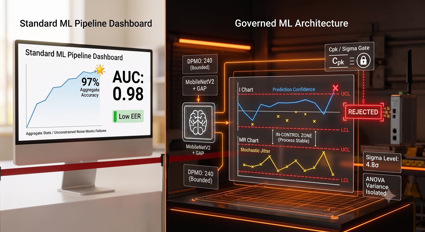
Here’s the reframe that matters: a model reporting 97% aggregate accuracy while remaining highly sensitive to environmental noise isn’t a strong model with an edge case. In production terms, it’s an out-of-control statistical process, one that generates hundreds of thousands of Defects Per Million Opportunities the moment it hits real conditions.
TRADITIONAL ML REPORTING (The Illusion):
[ Raw Input ] ──> [ CNN Model ] ──> "97% Aggregate Accuracy" ──> DEPLOYED (Hidden Field Failures)

GOVERNED ML ARCHITECTURE (The Fix):
[ Raw Input ] ──> [ MobileNetV2 + GAP ] ──> [ i-mR Control Chart ] ──> [ Cpk / Sigma Gate ] ──> CERTIFIED DEPLOYMENT
2. Bridging the gap: the DMAIC-GML protocol
The fix starts with a mindset shift. Deep learning inference stops being a one-time mathematical calculation and starts getting governed as a repeatable industrial process. Merge Lean Six Sigma’s Statistical Process Control with modern CNNs, and you get DMAIC-GML: Define, Measure, Analyze, Improve, Control, applied to Governed Machine Learning.
                     DMAIC-GML IMPLEMENTATION LIFECYCLE

  DEFINE         MEASURE        ANALYZE         IMPROVE        CONTROL
┌─────────┐    ┌─────────┐    ┌─────────┐    ┌─────────┐    ┌─────────┐
│ Formal  │ ──>│ 30-Run  │ ──>│ 2³ Full │ ──>│Structural│──>│Automated│
│ Defect  │    │Baseline │    │Factorial│    │Parameter │    │  i-mR   │
│ Mapping │    │  DPMO   │    │   DOE   │    │ Locking  │    │  Gate   │
└─────────┘    └─────────┘    └─────────┘    └─────────┘    └─────────┘
Here’s how each phase governs biometric and computer vision feature extraction.
Phase 1: Define, redefining biometric error
False Match Rate and False Non-Match Rate stop being the whole story. Every misclassification in a tracking sequence becomes a formally defined industrial Defect, and every inference pass counts as one Opportunity. That reframing lets DPMO get computed directly from the inference pipeline:
$$\text{DPMO} = \left( \frac{\text{Total Classification Defects}}{\text{Total Matching Opportunities}} \right) \times 10^6$$
Phase 2: Measure, establishing the operational baseline
Before any hyperparameter gets touched, a 30-run replicated baseline of the MobileNetV2 feature extractor runs under unconstrained environmental conditions. From that baseline, we calculate the Process Capability Index (Cpk) and the baseline process Sigma Level. If Cpk falls below 1.0, the process is statistically incapable of holding up operationally, no matter what the benchmark accuracy says.
Phase 3: Analyze, factorial root cause isolation
A 2³ Full Factorial Design of Experiments, combined with fixed-effects ANOVA, separates environmental sensor noise from genuine underlying variance. Three factors go into the test: embedding dimension (a low setting in the low hundreds vs. a high setting in the several-hundreds range), cosine margin penalty (a conservative low value vs. a more aggressive high value), and illumination augmentation (basic vs. Chebyshev histogram transformation). The analysis isolates main effects and interaction effects, pointing to which hyperparameter combination suppresses stochastic feature collapse.
Phase 4: Improve, interaction locking
Once ANOVA confirms which interaction terms actually matter, the optimal configuration gets locked in structurally. Combining Global Average Pooling with Chebyshev histogram pre-processing and a locked cosine margin penalty, for example, maximizes the separation between latent embeddings of visually similar subjects while cutting sensor drift.
Phase 5: Control, the i-mR governance gate
The deployment pipeline, hosted on GCP, sits behind an automated Individual-Moving Range control chart. The Individual (I) chart tracks rolling real-time prediction confidence; the Moving Range (MR) chart measures run-to-run jitter across sequential frames.
                  AUTOMATED i-mR GOVERNANCE GATE

  Moving Range (Jitter)
    │
UCL ├── ── ── ── ── ── ── ── ── ── ── ── (Upper Control Limit)
    │        x       x
    │  x   x   x   x   x   x  <── [In-Control Zone: Process Stable]
LCL ├── ── ── ── ── ── ── ── ── ── ── ── (Lower Control Limit)
    │                          X <── [Out-of-Control Signal: REJECTED]
    └─────────────────────────────────> Frame Sequence
The hard stop rule: if real-time inference capability drops below 3.0σ (Cpk < 1.0), the governance gate rejects the pipeline automatically. Low-confidence predictions get quarantined before they reach a downstream decision.
3. Standard ML vs. DMAIC-GML, side by side
| Architectural Metric | Standard Deep Learning Pipelines | DMAIC-GML Governed Architecture |
|---|---|---|
| Primary Evaluation Metric | Top-1 Accuracy, AUC, EER | Cpk (Process Capability), DPMO, Sigma Level |
| Noise Handling | Dynamic Data Augmentation (Trial & Error) | Fixed-Effects ANOVA Variance Isolation |
| Optimization Method | Manual Hyperparameter Tuning | 2³ Factorial Design of Experiments (DOE) |
| Deployment Gate | None (model serves all predictions) | Automated i-mR Control Chart Gate (rejects out-of-control frames) |
| Operational Reliability | High failure risk under environmental drift | Statistically bounded, reproducible inference |
4. What this means for production engineering teams
Test set accuracy alone tells you almost nothing about how a model behaves on edge hardware exposed to real environmental noise. High validation numbers and high field reliability are two separate claims.
DPMO gives engineering leads something a percentage can’t: an explicit, actionable reliability score, expressed the same way a manufacturing line would express it.
An i-mR control chart built directly into the inference pipeline is what turns “probably fine” into “statistically verified.” Only predictions that clear the gate reach a mission-critical end-user; everything else gets flagged before it can cause damage downstream.
Industrial quality control reshaped manufacturing in the 20th century. Deep learning is overdue for the same discipline in the 21st century.
Reference & Citation Notice
This blog post is adapted from doctoral research in Computer Science:
Akin-Tepede, Oladipupo. “Metric-Governed Error Modeling for Biometric Feature Stability.” PhD Dissertation, Department of Computer Science.
